CS 180 Project 4 - Image Warping and Mosaicing by Eshani Jha

Overview

In this project, I took a look into the fascinating process of image mosaicing by warping and stitching multiple photographs into seamless mosaics. Using manually selected correspondence points, I also aligned images through homography transformations. This technique not only allows for the creation of captivating panoramas, but also demonstrates how projective warping can be applied to rectify images to fit alternate perspectives.

Shoot the Pictures

For this project, I used my Samsung Galaxy S22+ to capture high-quality photographs with fixed frame rates and consistent lighting conditions. To create variety, I also incorporated video game screenshots by manually panning across different sections of the in-game map with my mouse, capturing individual screenshots to later stitch into a cohesive mosaic. The goal was to ensure that the transformations between images are projective (i.e., perspective transformations). This is typically achieved by fixing the center of projection and rotating the camera during capture. I took care to follow these principles to ensure smooth image alignment and warping.

Recover Homographies

To align the images in the mosaic, I used the same correspondence tool from Project 3 to manually label matching features between each pair of images. This process generated two sets of corresponding points: src_pts for the source image and dst_pts for the target image. Using these points, I computed the homography matrix following the Singular Value Decomposition (SVD) approach, as outlined in the referenced paper.

For each pair of correspondence points (x1, y1) and (x2, y2), two constraint vectors are created to form part of the system of equations:

            Vector 1: [-x₁, -y₁, -1, 0, 0, 0, x₁ · x₂, y₁ · x₂, x₂]
            Vector 2: [0, 0, 0, -x₁, -y₁, -1, x₁ · y₂, y₁ · y₂, y₂]
            

These vectors are derived by eliminating the scale factor w' in the target homogeneous coordinates, ensuring consistency across the transformation. The resulting vectors are stacked into a matrix A, which captures the relationship between the source and target points. Next, I passed matrix A through the SVD function np.linalg.svd(A), obtaining the matrices U, S, and VT. The row of VT (or the column of V) corresponding to the smallest singular value gives the solution vector v. This vector contains the elements of the flattened homography matrix.

Finally, I reshaped v into a 3 × 3 matrix H. To ensure the homography matrix is properly scaled, I divided each element of H by the value in its bottom-right corner. This normalized matrix H provides the transformation needed to warp the source image into the perspective of the target image.
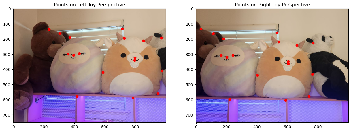
Points

Warp the Images

To align images into a seamless mosaic, I implemented a custom warping function that leverages a homography matrix to map the source image into the target perspective. The homography matrix transforms the corners of the source image, defining the new bounds and creating a pixel grid for the warped image. Using inverse mapping, each pixel in the target image is then traced back to its corresponding location in the source image. At these locations, I applied bilinear interpolation to compute smooth pixel values by blending the intensities of neighboring pixels. This ensures that the transitions between images are visually smooth and free of harsh boundaries.

The final warped images preserve spatial relationships and aligns accurately with the target image, setting the stage for blending multiple images into a unified mosaic.

Image Rectification

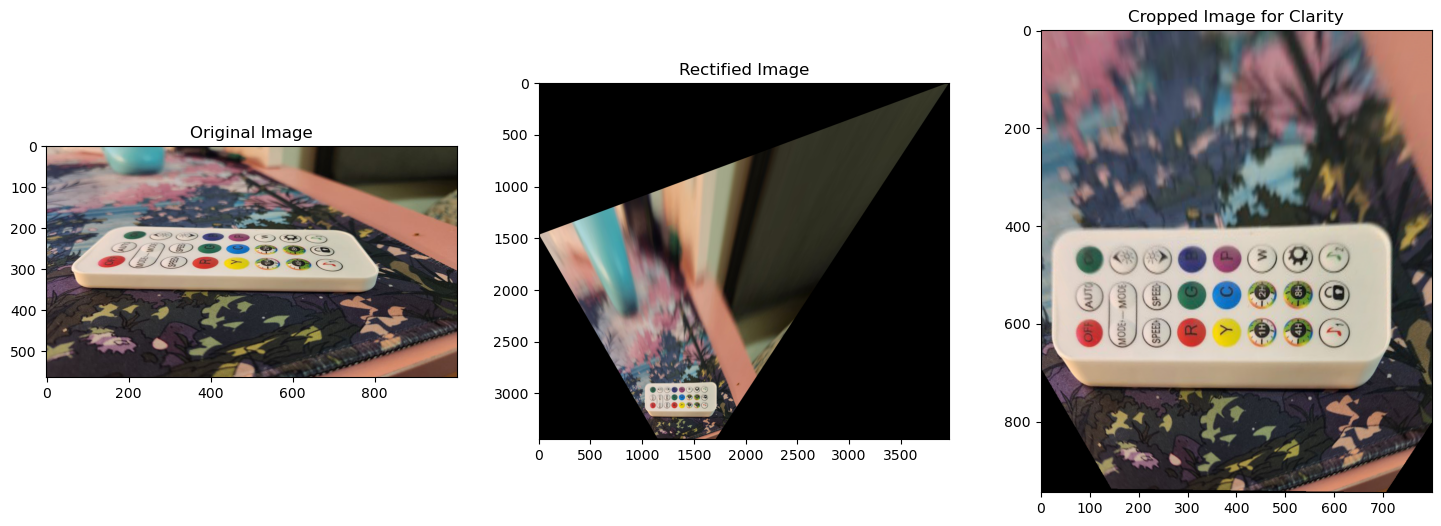
As part of testing the homography and warping functions, I performed image rectification on objects with known shapes. This process ensures that the code works correctly by transforming tilted or distorted objects back into their proper rectangular form. I captured images with objects such as my laptop screen and LED remote at an angle and used the homography transformation to "flatten" their appearance.

Interestingly, when rectifying the remote control, the transformation not only corrected the perspective but also revealed finer details that were initially hard to see. Surprisingly, symbols like the AUTO button and the W symbol (for white light) became clearly visible after rectification. This demonstrates the power of perspective correction in uncovering subtle features within an image.

Results

Laptop Remote

Blending into a Mosaic

First, I computed a homography matrix to warp one image onto the plane of another. Then, I calculated the bounding box and necessary shifts to align the warped image with the target image. Finally, both images were stitched together within the mosaic by placing them at their computed positions in the combined frame.

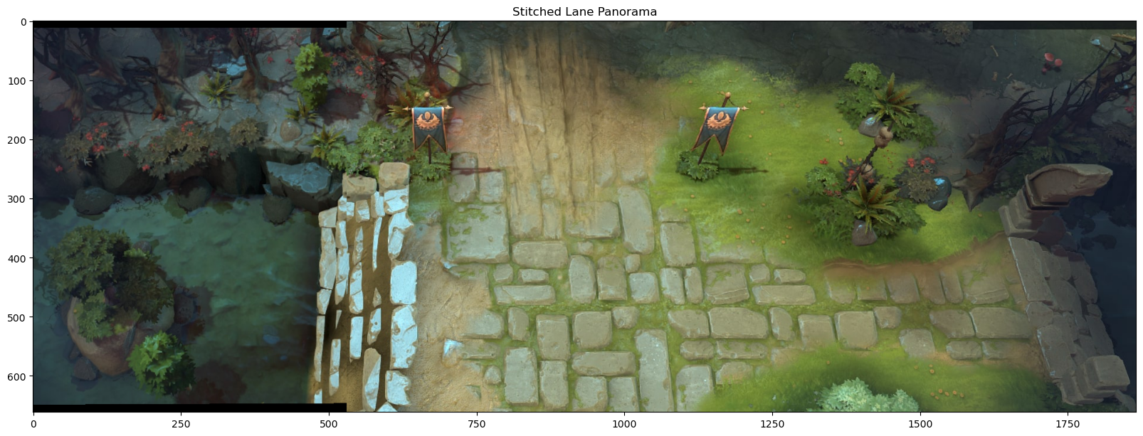
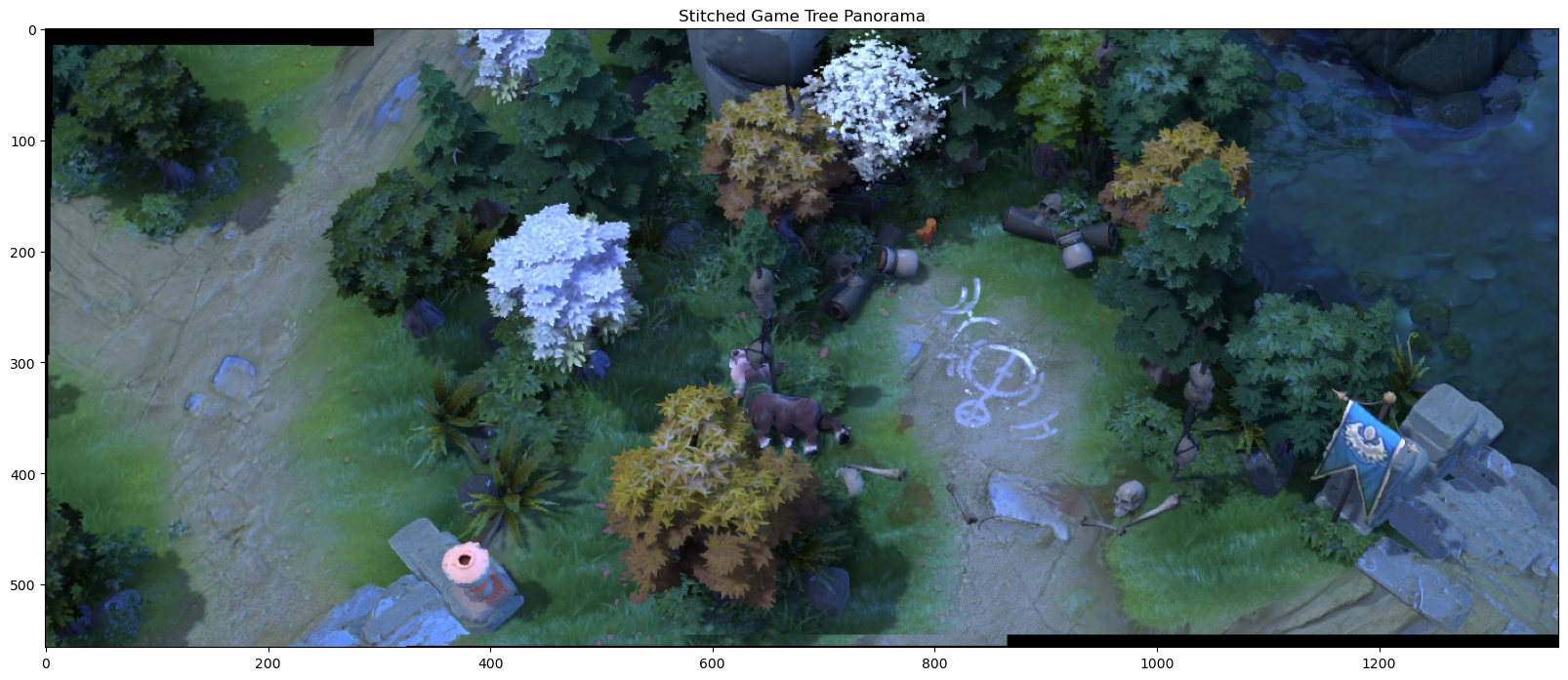
I applied this process to create a mosaic of stuffed animals (real-world example) and used blending techniques to eliminate sharp edges. I also experimented with Dota 2 screenshots to explore how parts of a video game map look on a larger scale, as the in-game view is limited. I tested the process on different landscapes, including the “lane,” which contains mostly similar textures, and the “trees,” which have intricate leaf details.

Real-Life Results

Toy Panorama

Game Results (Lane)

Dota Dota

Game Results (Trees)

Tree Tree

Detecting Corner Features

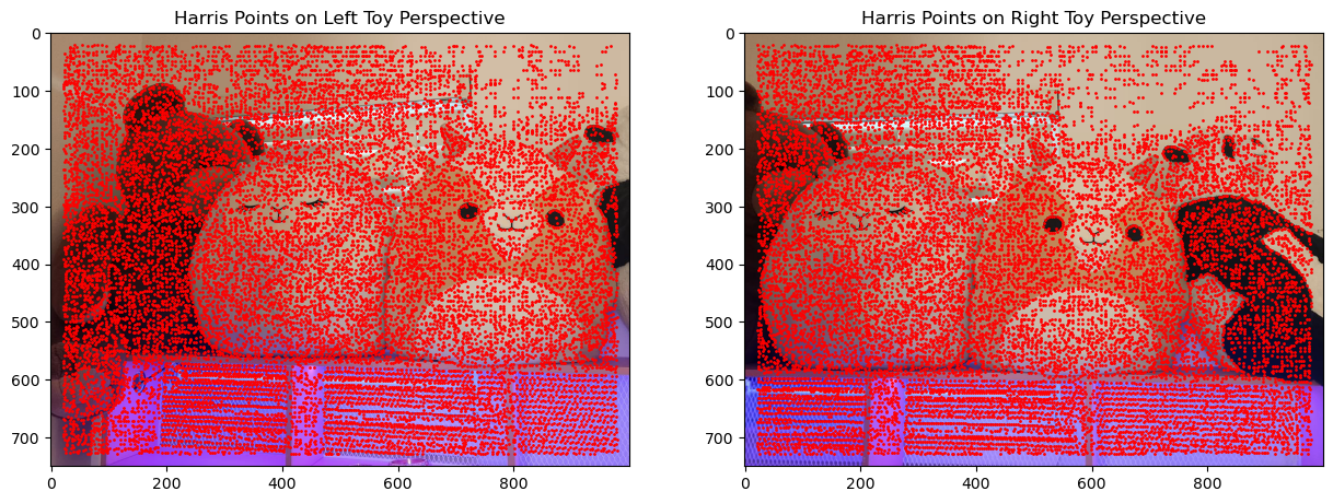
In Part A, I manually selected correspondence points to compute the homography matrix. Later, I automated this process by implementing the Harris Corner Detector, which identifies interest points, or corners, within an image. A corner is a point where two edges meet, creating a significant change in brightness, and Harris corners are reliable for feature detection as they are invariant to translation, rotation, and illumination changes.

The detector calculates the structure tensor \( M \) using image derivatives in the x and y directions. Each window is scored using \( R = \det(M) - k(\text{trace}(M))^2 \), where the eigenvalues of \( M \) determine if the region contains a corner, edge, or flat area. I applied the Harris detector to both the left and right images to extract key corner features automatically.

Results

Toy Panorama

Adaptive Non-Maximal Suppression (ANMS)

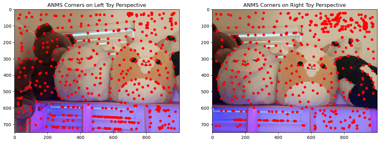
While the Harris Corner Detector identifies many potential feature points, it often produces too many. To address this, Adaptive Non-Maximal Suppression (ANMS) filters the points by distributing them evenly across the image, keeping only the strongest features. ANMS calculates a suppression radius for each point defined as the smallest distance to a significantly stronger point using a robustness parameter \(c = 0.9\).

The algorithm works by computing the Euclidean distance and strength differences between each point and others. Points with non-positive strength differences are discarded. The nearest valid distance is stored in a min-heap, which maintains the largest suppression radii. While ANMS may not return the points with the highest strengths, it ensures that the selected features are spatially well-distributed, providing strong, dominant points across the image. The final set of Harris points is shown below.

Toy Panorama

Extracting Feature Descriptors

With a reduced set of Harris points, the next step is to match points between images using feature descriptors. Each descriptor is created by extracting a 40x40 window centered on a Harris point. This patch captures a 20-pixel radius around the point in all directions. To generate a smooth, blurred descriptor, the patch is downsampled to 8x8 pixels instead of extracting a smaller patch directly.

The descriptors are then normalized to have a mean of 0 and a standard deviation of 1, making them robust to affine changes in intensity (e.g. bias and gain). These normalized feature descriptors allow consistent and reliable matching between images.

Matching Feature Descriptors

To match feature descriptors, we compare all descriptor pairs between the two images using Sum of Squared Differences (SSD) or Nearest-Neighbor (NN) scores, where lower scores indicate better matches. We first narrow the candidates by selecting each feature’s nearest neighbor. Next, we calculate the ratio between the nearest-neighbor score and the second-nearest-neighbor score. If this ratio is below a chosen threshold (0.4 worked well in my testing), we accept the match. The resulting matches are visualized with randomly colored points to highlight correspondences between the images.

Results

Even though some mismatches remain, the majority of the matches are accurate and reliable.

Toy Panorama

RANSAC

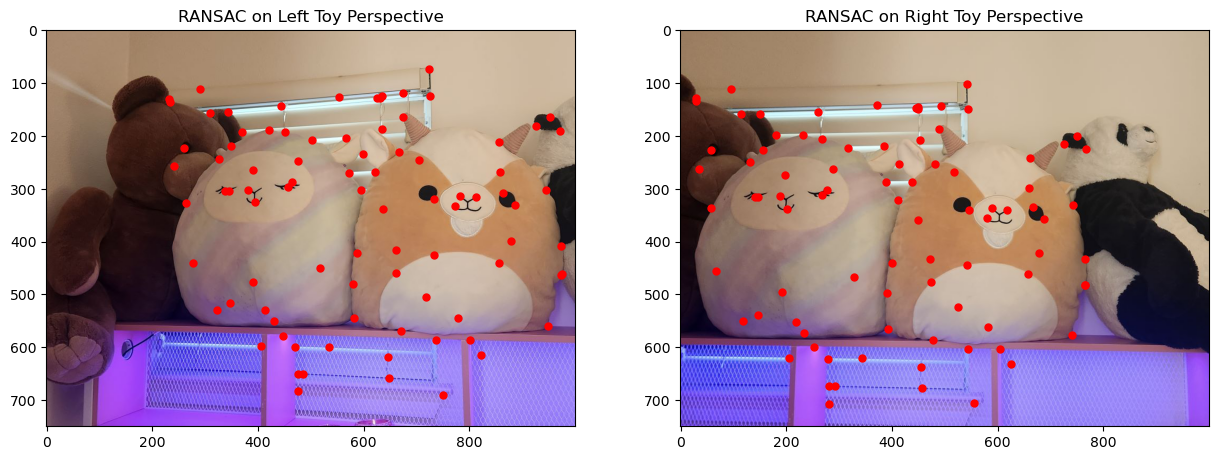
To eliminate false positives from the feature matching process, we apply RANSAC. In each iteration, a random set of 4 matches is selected to compute a homography. We then evaluate how well this homography aligns the remaining matches, counting the number of inliers it produces. The homography with the highest number of inliers is selected as the final result. While some true matches may be lost, most correct matches are retained. Also, all incorrect matches are removed which leads to more reliable stitching.

Results

Toy Panorama

Blending into a Mosaic

I used the same techniques as Part A. First, I computed a homography matrix to warp one image onto the plane of another. Then, I calculated the bounding box and necessary shifts to align the warped image with the target image. Finally, both images were stitched together within the mosaic by placing them at their computed positions in the combined frame.

I applied this process to create a mosaic of stuffed animals (real-world example) and used blending techniques to eliminate sharp edges. I also experimented with Dota 2 screenshots to explore how parts of a video game map look on a larger scale, as the in-game view is limited. I tested the process on different landscapes, including the “lane,” which contains mostly similar textures, and the “trees,” which has intricate leaf details.

Real-Life Results

Below are my manually and automatically stitched results side by side. They both appear to be similar.

Toy Panorama

Game Results (Lane)

Below are my manually and automatically stitched results side by side. They both appear to be similar.

Dota

Game Results (Trees)

Below are my manually and automatically stitched results side by side. The automatic stitching noticeably outperformed the manual approach, as evidenced by the absence of a shadow artifact along the bottom edge in the automatically stitched image (around 650 on the horizontal axis). This comparison highlights the precision and effectiveness of the automated process.

Tree

What I learned

The most mind-blowing part of this project has been discovering the power of feature matching based solely on pixel intensities. I had always assumed that recognizing similar points across images required a neural network or some form of “smart” AI to make sense of it all. But seeing how pixel intensities alone can accurately pinpoint matching features between images was eye-opening! It felt like unlocking a new layer of understanding in computer vision—realizing that the simplest data can sometimes yield the most precise results.